Finding Flowers with Neural Networks

So, somewhere there is a great beginning to a very detailed post about gradient descent and supervised learning. And I cannot for the life of me find it! I got busy with this month - two projects for the term down, and one to go. So if I find that post, I'll post it (or maybe I'll write a different one) but in the meantime I wanted to post on the project I've just done.
This was quite a feat of learning and programming for me and I'm pretty happy with the results. What did I do, I used deep learning, or neural networks, to take an image of a flower and predict it. It's just a tiny bit fancy. :P
What is Deep Learning?
As usual, before I get into the details of the project, it's a good idea to explain what we were actually doing. We've been talking about machine learning right? And we talked about how we use algorithms to understand the data? (Trust me, we did - you can go back and refer to the link if you are unsure!) Well, in deep learning we discover just how powerful that concept can be!
What we do in deep learning is we make many algorithms (they can be simple or less simple) and we connect them together. Hmm, you know what could help us here? A picture. So, here we go:
The Structure
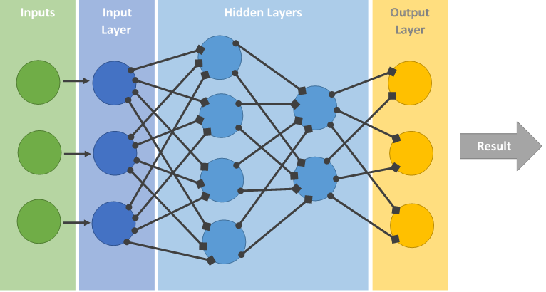
To be honest, you'd be forgiven if your first response upon looking at it was, "This is a criss-crossed mess!" But if you take the time to follow everything through (I put markers at the end of the lines to help with counting) you will find that each circle in one column connects to each circle in the next column. (HINT: To easily check this, if you count up the number of circles in the previous column, there should be that many squares touching each circle.) This is what we would call a fully-connected (there are others that are not) sequential neural network.
It's important to point out that there is nothing required about the exact numbers here - it's possible to have as many circles as you like in the hidden layers, and as many hidden layers as you would like, or none. It ends up being about what makes the most sense for your curent situation. (And working this out can be somewhat arbitrary)
Oh, also, the technical term for the large circles is actaully nodes. So I'm going to start using that term. :)
The Input Layer
So here's how it works. In this case we can say that we have three details about which we have information on for every data point we have. These are out inputs and will be fed into the input layer. To be honest, the input layer, as I've described it here, is not like any other layer in the network. It's only job is to collect the inputs. It will always have the same number of nodes as there are data inputs. Normally there are a whole bunch of other things that happen before the data gets passed into a layer, but I'll describe that below.
When we start out, we will weight each detail as it is fed into the node. Usually, these are just random (but probably close to zero), and we can talk about them existing on the lines, or the edges. There is a different weight for each input for each node in the input layer.
The Hidden Layers
After the gathering of the input layer, we then feed the data through the internal network. Each of these is called a hidden layer. When data is passed into a node in the hidden layer, it is weighted (multiplied) by a certain value. Usually, these are just random (but probably close to zero), and we can talk about them existing on the lines, or the edges. There is a different weight for each type of data received by each node.
At the node we will multiply the values by the weights on the edges and then do a fancy transformation (called an activation) of the numbers that will convert them (typically) to their equivalent in a range of:
- Between 0 and 1 (sigma/sigmoid)
- Between -1 and 1(tanh), or
- Between 0 and all positive numbers (ReLU)
We will then take these newly calculated values and do the same thing. We'll feed the information into the nodes of the next layer (in our case a hidden layer with four nodes), again, multiplying them by random edge weights, and converting them to the new scale. We will keep doing this until we get to the final layer, the output layer.
The Output Layer
The output layer needs to be the same size as the number of categories that we have. In our case, we have three different categories that we are trying to predict, but don't be confused - the number of output nodes does not need to match the number of input nodes, it just did in this case. The number of input nodes is determined by the number of pieces of information we have for each data point, the number of output nodes is determined by the number of categories we need to predict.
At the output layer, we do the same multiplying by weights thing, but this time we specifically use the sigma(for two categories)/sigmoid(for more than two categories) activation. The reason that we do this is that we do this is that it will give us the equivalent of a probability that the piece of data is that particular category. So, in our case, with three categories, the results would give us three values for any data point, one for the probability of it being in the first category, one for the probability of it being in the second, and one for it being in the third.
We are getting there! The final thing that we do in this process is to compare our predictions to what is actually there. We take the category that had the highest probability and compare it to what we know the actual result is. (For a supervised learning model - which this is - we need to know what the result is supposed to be) We then measure our predictions against the results and note which ones we got right and which ones we didn't. We'll select a specific measure to determine exactly how we're measuring how well we did. This whole process is called feedforward.
Backpropagation
To get the model to actually learn, we then take this information and feed it backwards through the results. We do this by working out how to distribute the contribution to the errors throughout the network. Based on this, we then update the weights. And then we just keep repeating this many times over.
The data points can go through one at a time, or go through collectively. Often, what is done to go through in small sets of data, called mini-batching.
The Project
So what did I do for the project? For the project itself, the data points we were classifying were images of flowers that come from this resource. This is managed with algorithms by converting each of the pixels to their numeric code for their position and their colour.
You then do what is described above, set up the network architecture, run the pictures through multiple times and see if it gets better. We were required to include the ability to print out the ongoing changes in the error rates and the accuracy of predicting a validation set of images. (Not the same ones that the algorithm trained on) I must say, I think you can truly claim AI nerd status when one of the things you can't help but do is stare at the improving accuracy of your model, and verbally cheer it on with calls of, "You can do it!" Yes, I really am that person.
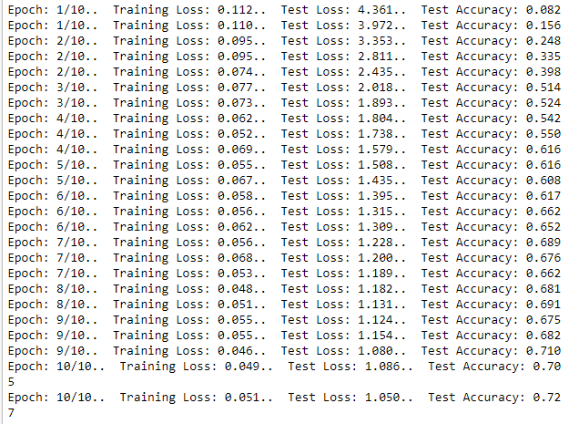
For some more technical details, I chose the vgg19_bn (for more info on the vgg models you can check out this architecture post) through a recommendation from StackOverflow. In our supervised learning classes we had learnt about using grid search to identify the best model setup (Identifying a possible range of parameters and then testing each combination) but had also read that a random search (randomly picking the values) can be more effective. So I set up a basic function used three different optimizers (what informs how changes to the weights are implemented - this article provides an amazing overview/summary), learning rates (informs how big each change will be), and epochs (the number of times the dataset is run through the model for training). The best results in terms of prediction accuracy were an Adam optimizer (makes different changes on the weights in the based on frequency of the associated input features, contributes some of the previous information about changes in both a squared and linear manner), with a learning rate of 0.0003089 and 28 epochs. In terms of validation accuracy (predicting previously unseen images), it reached around 85% accuracy at 22 epochs. The model was trained for another 30 epocs with reducing learning rates but only improved its accuracy by about 3%.
Ok, enough technical details, here's what it actually did!
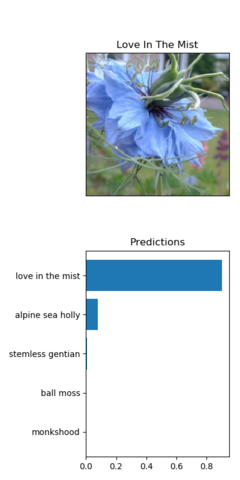
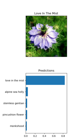
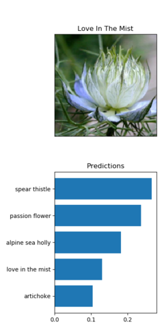
What I find most interesting about this group of flowers is that even at different angles, the predictions for this flower are above 80%. However, it looks like most of these images are for older flowers, and the final, seemingly newer bloom is what confuses the algorithm. To the human eye, this definitely would not be considered a spear thistle or passion flower, but the correct flower type is in the list.
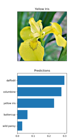
I also enjoyed looking at what other flowers were predicted and some of their similarities, and the flow-ons from there:
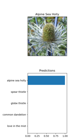

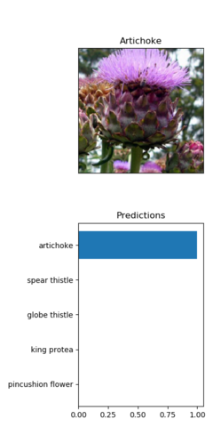
I find it both amazing how the predictions seem to be able to pick up the visual similarities between the images (in that these are the next most probable flower types) but also that it can so clearly distinguish between the differences (with high probabilities for each classification)
It's also then fascinating to notice when this doesn't happen - when the model can't reliably identify a flower type:
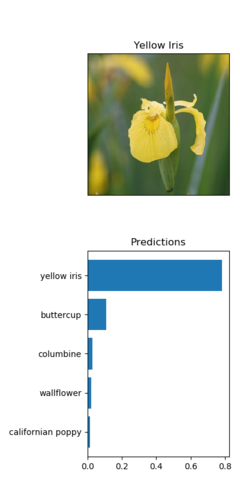
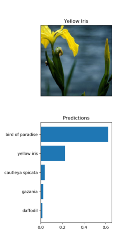
It seems like the clarity of the image, the fullness of the image in the frame, and the features that are captured could play a role in accurate detection.
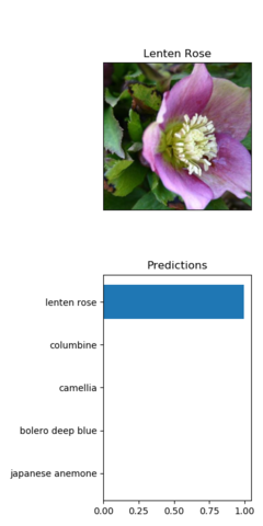
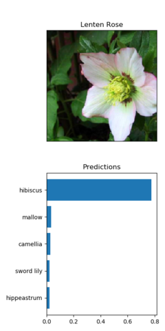
Also equally fascintating when seemingly different flowers can all be correctly classified, such as the lenten rose.
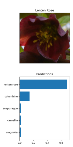
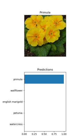
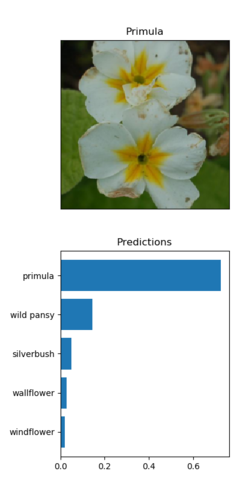
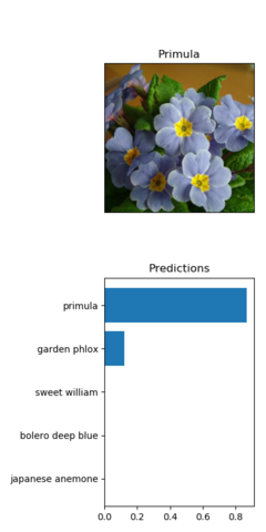
Well, it does get one wrong. But there's also the primula:
To be able to improve the accuracy, I could have trained the algorithm more, but another way that I could have improved it would have been to identify what types of flowers, or image types the algorithm particularly struggled with and find more of those to help it train on. I really did enjoy this project - it was an education in both the process of deep learning and the a variety of coding practices required. If you'd like to check it out in more detail, you can head here.